Get started

Use cases.

Load data

# Read *.ods or excel (spreadsheet).
data = pd.read_excel('D:\...\data2.ods', sheet_name=0,
                     skiprows=1).dropna(how='all')
data.name = 'data2'

Experiment subpackage

You can either use subpackages directly (physicslab.experiment.van_der_pauw) or utilize the following batch function.

# Example: Van der Pauw
import pandas as pd

def load(filename):
   data = pd.read_csv(filename + '.csv')
   data.name = filename
   return data

thickness = 1.262e-6  # meters
samples = ['sample#1', 'sample#2', ...]
data_list = [load(sample) for sample in samples]

results = physicslab.experiment.process(
   data_list,
   by_module=physicslab.experiment.van_der_pauw,
   thickness=thickness
)
print(results)

           sheet_resistance  ratio_resistance  sheet_conductance  resistivity  conductivity
units       ohms per square                 1      1/ohms square        ohm m       1/ohm/m
sample#1       1.590823e+05          1.168956       6.286055e-06     0.200762      4.981026
sample#2       1.583278e+05          1.185031       6.316009e-06     0.199810      5.004762
...

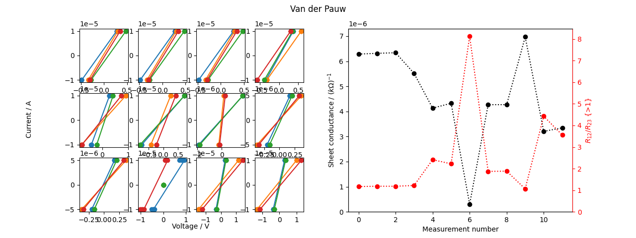
Van der Pauw

Handling Geometry enum.

def get_geometry(orientation, direct):
   """
   :param int orientation: Contacts rotation in multiples of 90°.
   :param bool direct: Contacts counter-clockwise (True) or not.
   """
   geometry = van_der_pauw.Geometry.R1234  # Default configuration.
   geometry = geometry.shift(number=orientation)
   if not direct:
      geometry = geometry.reverse_polarity()
   return geometry

Plotting.

from physicslab.experiment import van_der_pauw

data_list = load(sample_name)  # Custom function.
results = physicslab.experiment.process(data_list, by_module=van_der_pauw)
van_der_pauw.plot(data_list, results)
plt.show()

Magnetism type

results = physicslab.experiment.magnetism_type.process(measurement)
print(results)

cols = physicslab.experiment.magnetism_type.Columns
B = measurement[cols.MAGNETICFIELD]
plt.plot(B, measurement[cols.MAGNETIZATION], 'ko')  # Original data.
plt.plot(B, measurement[cols.DIAMAGNETISM], 'r-')  # Separated DIA contribution.
plt.plot(B, measurement[cols.FERROMAGNETISM], 'b-')  # Separated FM contribution.
plt.plot(B, measurement[cols.RESIDUAL_MAGNETIZATION], 'g-')  # Residual (unseparated) data.
plt.show()

curves.Line

line1 = Line(3, -2)  # Line: y = 3 - 2x
line2 = Line(slope=2)  # Line: y = 0 + 2x
line1(4.3)  # -5.6
line1 - 5.3 + 2.4 * line2  # Line: y = -2.3 + 2.8x
line1.zero()  # 1.5
Line.Intersection(line1, line2)  # (0.75, 1.5)

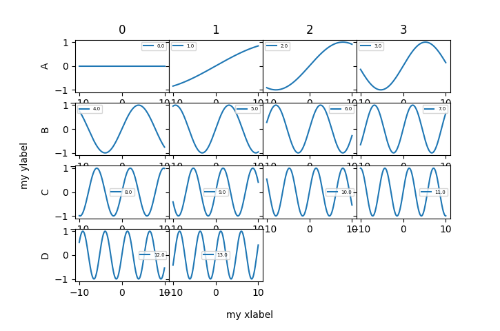
ui.plot_grid & utility.squarificate

import matplotlib.pyplot as plt
import numpy as np
import physicslab

x = np.linspace(-10, 10, num=1000)

def plot_value(ax, value):  # Sine.
   ax.plot(x, np.sin(x * value / 10), label=value)

def alphabet(num):  # ['A', 'B', ...]
   return [(chr(ord('A') + i)) for i in range(num)]

data = np.arange(14, dtype=float)  # E.g. a list of measurements.
data = physicslab.utility.squarificate(data)  # Squarish 2D array distribution.
df = pd.DataFrame(data, index=alphabet(data.shape[0]))  # Naming.
df.name = 'My title'

print(df)
physicslab.ui.plot_grid(
   df, plot_value, xlabel='my xlabel', ylabel='my ylabel',
   subplots_adjust_kw={'hspace': 0}, sharey=True, legend_size=5)

      0     1     2     3
A   0.0   1.0   2.0   3.0
B   4.0   5.0   6.0   7.0
C   8.0   9.0  10.0  11.0
D  12.0  13.0   NaN   NaN

Show images

import matplotlib.image as mpimg

# Show pictures (like SEM images). Parameter value is then e.g. a filename.
def plot_value(ax, value):
   img = mpimg.imread(filepath)
   ax.imshow(img, cmap='gray')